Measures of Central Tendency
Measures of Central Tendency
Introduction
"Central tendency" answers the question: what is a typical value in this dataset? Three classic answers exist: the mean, the median and the mode. Choosing the wrong one misleads your audience - especially with skewed data.
The Mean (Average)
The sum of all values divided by the count:
mean = (x1 + x2 + ... + xn) / n
import numpy as npsalaries = np.array([3200, 3400, 3500, 3600, 3800, 4100, 25000])
print(f"mean salary: {salaries.mean():.0f}")
Output:
mean salary: 6543
The mean is dragged upward by the single 25,000 salary. Is 6,543 a fair "typical" salary? Probably not - the boss's salary distorts the picture.
The Median
The middle value when data is sorted. With an odd count it is the center value; with an even count, the average of the two middle values.
salaries = np.array([3200, 3400, 3500, 3600, 3800, 4100, 25000])
print(f"median salary: {np.median(salaries):.0f}")
Output:
median salary: 3600
The median ignores extreme values. For income, house prices, or rental costs, the median is usually the honest choice.
The Mode
The most frequent value. Useful mainly for categorical and discrete data.
from collections import Counter
ratings = [5, 4, 5, 3, 5, 4, 2, 5, 3, 4]
print(Counter(ratings).most_common(1))
Output:
[(5, 4)]
A dataset can have two modes (bimodal) or more. A histogram with two peaks often signals two different subgroups hiding in the data.
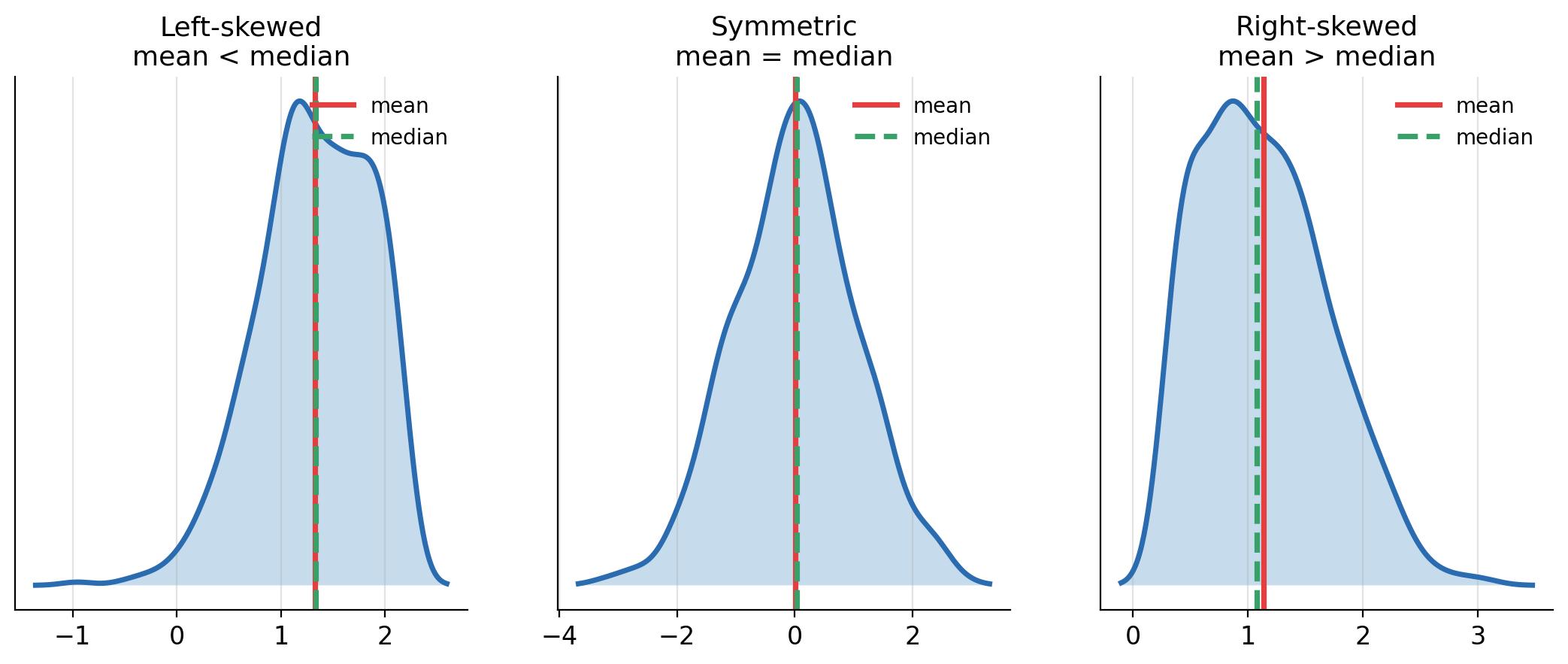
Skewness: When Mean and Median Diverge
- Symmetric: mean ≈ median ≈ mode.
- Right-skewed (positive): long tail on the right; mean > median.
- Left-skewed (negative): long tail on the left; mean < median.
Example: Order Values
import numpy as nprng = np.random.default_rng(7)
orders = np.concatenate([rng.normal(45, 8, 350), rng.normal(70, 6, 150)])
print(f"mean:   {orders.mean():.2f}")
print(f"median: {np.median(orders):.2f}")
Output:
mean:   52.50
median: 48.20
The mean is 4.30 higher than the median because of the premium segment in the right tail.
When to Use Which
| Situation | Best measure |
|---|---|
| Symmetric data, no outliers | Mean (uses all information) |
| Skewed data, income, prices | Median (robust to outliers) |
| Categorical data | Mode |
| Need further math (variance, tests) | Mean |
Weighted Mean
When groups have different sizes, the overall average is a weighted mean:
# 350 regular orders (avg 45) + 150 premium orders (avg 70)
weighted = (350  45 + 150  70) / 500
print(f"weighted mean: {weighted:.1f}")
Output:
weighted mean: 52.5
Common Pitfalls
- Reporting the mean for skewed data without checking the histogram.
- Forgetting outliers exist (always compute mean AND median).
- Using the mean for ordinal data (a "mean rating" of 3.7 is shaky math).
Summary
- Mean: sensitive to outliers, great for symmetric data.
- Median: robust, best for skewed distributions.
- Mode: only real option for categorical data.
- Compare mean and median to detect skewness quickly.
Next Lesson
Next up: measures of spread - how to quantify variability with range, variance, standard deviation and the IQR.
Quiz - Quiz - Measures of Central Tendency
1. Which measure is most affected by outliers?
2. For skewed income data, which measure best represents the typical case?
3. If mean > median, the distribution is likely:
4. The mode is the value that:
5. A bimodal histogram (two peaks) often signals: