The Normal Distribution and Z-Scores

Introduction

The normal (Gaussian) distribution is the workhorse of statistics. Many real-world variables - heights, measurement errors, test scores, product weights - are approximately normal. It is also the distribution that sample means converge to, which makes it the engine behind confidence intervals and hypothesis tests.

The Bell Curve

A normal distribution is described by two parameters:

• Mean mu: where the peak is.
• Standard deviation sigma: how wide the curve is.

The Empirical Rule (68-95-99.7)

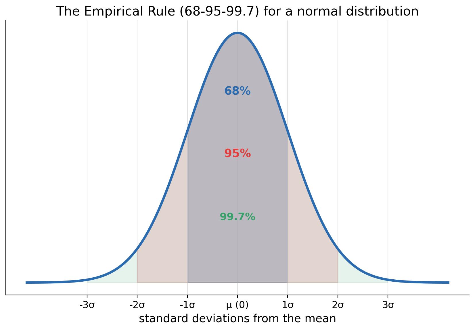
For any normal distribution:

• About 68% of values fall within 1 standard deviation of the mean.
• About 95% fall within 2 standard deviations.
• About 99.7% fall within 3 standard deviations.

import numpy as np
from scipy import stats
mu, sigma = 100, 15   # e.g. IQ scores
for k in [1, 2, 3]:
    pct = stats.norm.cdf(mu + k  sigma, mu, sigma) - stats.norm.cdf(mu - k  sigma, mu, sigma)
    print(f"within {k} sigma: {pct*100:.1f}%")

Output:

within 1 sigma: 68.3%
within 2 sigma: 95.4%
within 3 sigma: 99.7%

Z-Scores: Standardizing

A z-score tells you how many standard deviations a value is from the mean:

z = (x - mu) / sigma

iq = 130
z = (iq - 100) / 15
print(f"z = {z:.2f}")

Output:

z = 2.00

An IQ of 130 is 2 standard deviations above the mean - better than about 97.7% of the population.

Finding Probabilities with the CDF

The cumulative distribution function (CDF) gives the probability of being at or below a value.

from scipy import stats
P(IQ < 115) for IQ ~ N(100, 15)
p = stats.norm.cdf(115, 100, 15)
print(f"P(IQ < 115) = {p:.3f}")
P(IQ > 130)
p_above = 1 - stats.norm.cdf(130, 100, 15)
print(f"P(IQ > 130) = {p_above:.3f}")

Output:

P(IQ < 115) = 0.841
P(IQ > 130) = 0.023

Inverse: Finding the Value for a Percentile

The inverse CDF (percent point function) answers: which value cuts off the top 10%?

# Value with 90% of the population below it
q90 = stats.norm.ppf(0.90, 100, 15)
print(f"90th percentile IQ = {q90:.0f}")

Output:

90th percentile IQ = 119

Why the Normal Distribution Matters So Much

1. Many measurements are approximately normal (central tendency of errors). 2. Sample means become normal regardless of the population shape (Central Limit Theorem - next lesson). 3. Statistical tests (t-tests, ANOVA) assume normality; with large samples, the CLT makes this assumption safe.

Checking Normality

Quick visual check: a histogram with a smooth bell shape, or a Q-Q plot.

import matplotlib.pyplot as plt
from scipy import stats
data = np.random.normal(100, 15, 300)
stats.probplot(data, dist="norm", plot=plt)
plt.title("Q-Q plot: points near the line = approximately normal")
plt.tight_layout(); plt.show()

If the points stay close to the diagonal line, the data is approximately normal.

Common Pitfalls

• Assuming every dataset is normal - check first! (Income, prices and counts are often skewed.)
• Confusing the empirical rule with exact values (68.27%, 95.45%, 99.73%).
• Forgetting to use the standard deviation of the sampling distribution for means, not the data's sigma.

Summary

• Normal distributions are defined by their mean and standard deviation.
• 68-95-99.7 rule: one, two, three standard deviations.
• Z-scores standardize any value: z = (x - mu) / sigma.
• CDF gives probabilities; PPF gives percentile values.
• Always verify normality before assuming it.

Next Lesson

In the next lesson you will see why normal distributions appear everywhere: sampling distributions and the Central Limit Theorem.