Measures of Spread
Measures of Spread
Introduction
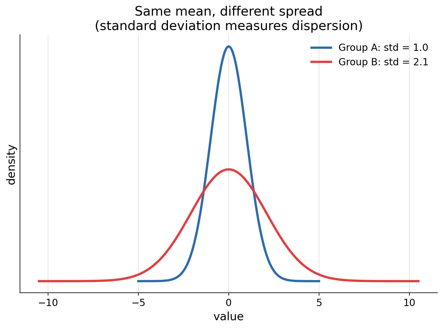
The average tells you the center, but not how varied the data is. Two classes can both average 70% on an exam while one has everyone at 69-71% and the other has students from 30% to 100%. Measures of spread quantify that variability.
Range
The simplest measure: max minus min.
import numpy as npgroup_a = np.array([69, 70, 70, 71, 70])
group_b = np.array([30, 55, 70, 85, 100])
print(f"A: range = {group_a.max() - group_a.min()}")
print(f"B: range = {group_b.max() - group_b.min()}")
Output:
A: range = 2
B: range = 70
The range is easy but fragile: a single outlier changes it completely.
Variance
The average squared distance from the mean. Squaring removes the sign and punishes large deviations.
variance (population) = sum((xi - mean)^2) / n
variance (sample)     = sum((xi - mean)^2) / (n - 1)
The sample version divides by n-1 (Bessel's correction) because a sample slightly underestimates the true spread.
print(f"A: variance = {group_a.var(ddof=1):.2f}")
print(f"B: variance = {group_b.var(ddof=1):.2f}")
Output:
A: variance = 0.70
B: variance = 742.50
Standard Deviation
The standard deviation is the square root of the variance. It brings the measure back to the original units - this is the number people quote as "sigma".
print(f"A: std = {group_a.std(ddof=1):.2f}")
print(f"B: std = {group_b.std(ddof=1):.2f}")
Output:
A: std = 0.84
B: std = 27.25
Quartiles and the Interquartile Range (IQR)
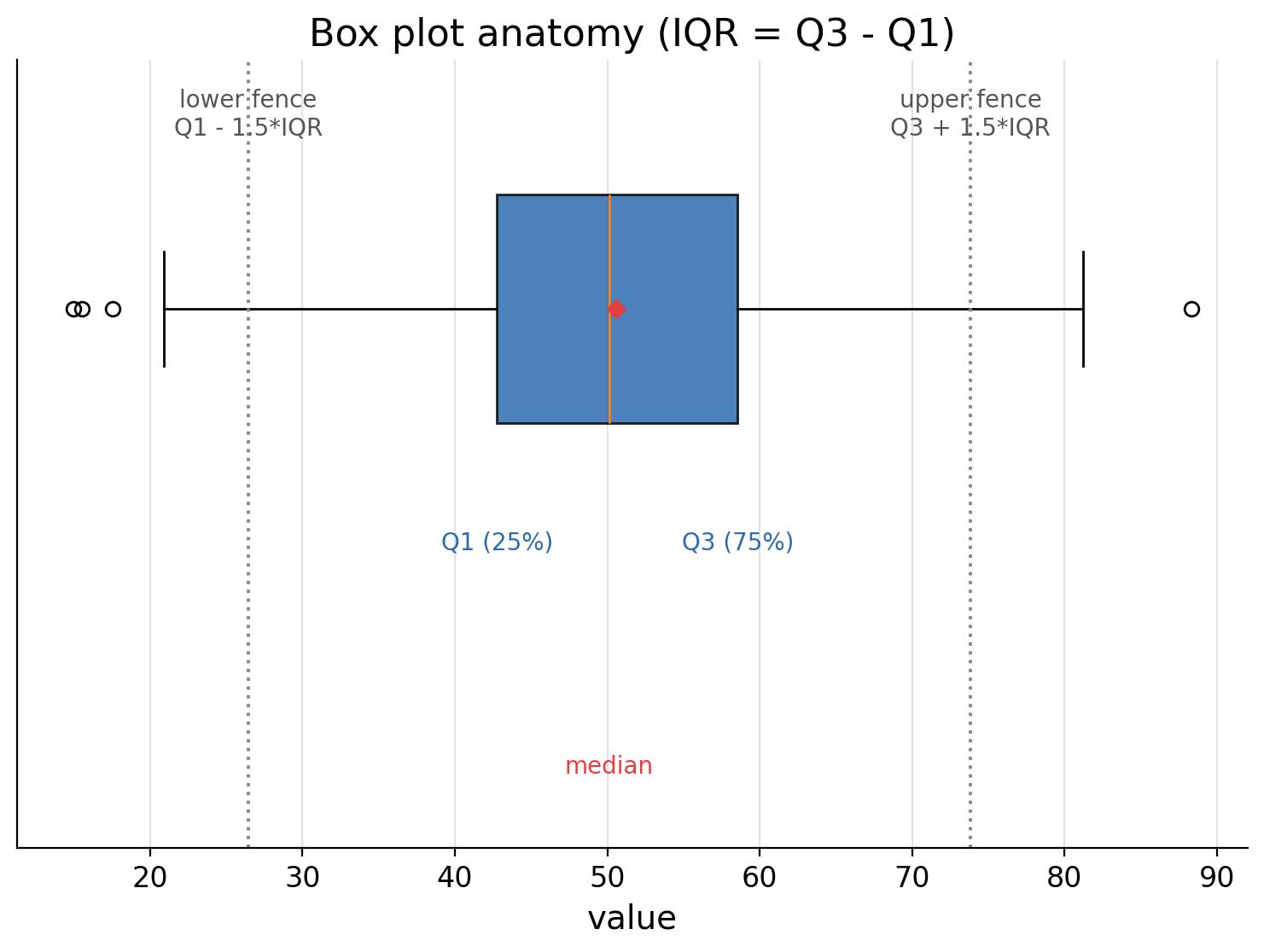
The median splits data in half. Quartiles split it into quarters:
- Q1: 25th percentile (median of the lower half)
- Q2: median (50th percentile)
- Q3: 75th percentile (median of the upper half)
- IQR = Q3 - Q1: the middle 50% of the data
import numpy as np
data = np.array([10, 12, 14, 15, 16, 18, 21, 22, 24, 30, 45])
q1, q3 = np.percentile(data, [25, 75])
print(f"Q1 = {q1}, Q3 = {q3}, IQR = {q3 - q1}")
Output:
Q1 = 14.5, Q3 = 24.0, IQR = 9.5
Outliers: The 1.5 x IQR Rule
A common rule flags values as outliers if they fall outside:
Q1 - 1.5 IQR or Q3 + 1.5 IQR
lower_fence = q1 - 1.5 * (q3 - q1)
upper_fence = q3 + 1.5 * (q3 - q1)
outliers = data[(data < lower_fence) | (data > upper_fence)]
print(f"outliers: {outliers}")
Output:
outliers: [45]
Variance vs Standard Deviation vs IQR
| Measure | Units | Robust to outliers? | Use case |
|---|---|---|---|
| Range | original | No | Quick look |
| Variance | squared units | No | Math, modeling |
| Std deviation | original | No | Reporting spread |
| IQR | original | Yes | Box plots, skewed data |
Coefficient of Variation
To compare spread across datasets with different means, use the coefficient of variation:
cv_a = group_a.std(ddof=1) / group_a.mean()
cv_b = group_b.std(ddof=1) / group_b.mean()
print(f"CV A = {cv_a:.3f}, CV B = {cv_b:.3f}")
Output:
CV A = 0.012, CV B = 0.389
Common Pitfalls
- Quoting variance in squared units (salary squared makes no sense).
- Using the range as the main spread measure.
- Forgetting to use ddof=1 for sample data in numpy.
Summary
- Range: quick but fragile.
- Variance: average squared deviation; sample version divides by n-1.
- Standard deviation: variance in the original units.
- IQR: robust middle-50% measure, used in box plots and outlier rules.
- Compare spread across groups with the coefficient of variation.
Next Lesson
Now that you can measure center and spread, the next lesson shows how to present data visually: histograms, box plots, bar charts and scatter plots.
Quiz - Quiz - Measures of Spread
1. The standard deviation is:
2. Why does sample variance divide by n-1 instead of n?
3. The IQR (interquartile range) measures:
4. Which measure is most robust to outliers?
5. A value is flagged as an outlier if it exceeds: